CPSC 340 Decision Trees

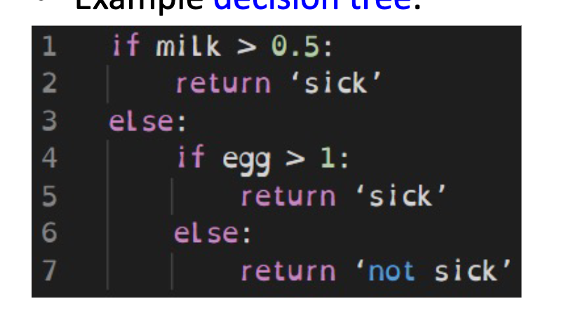
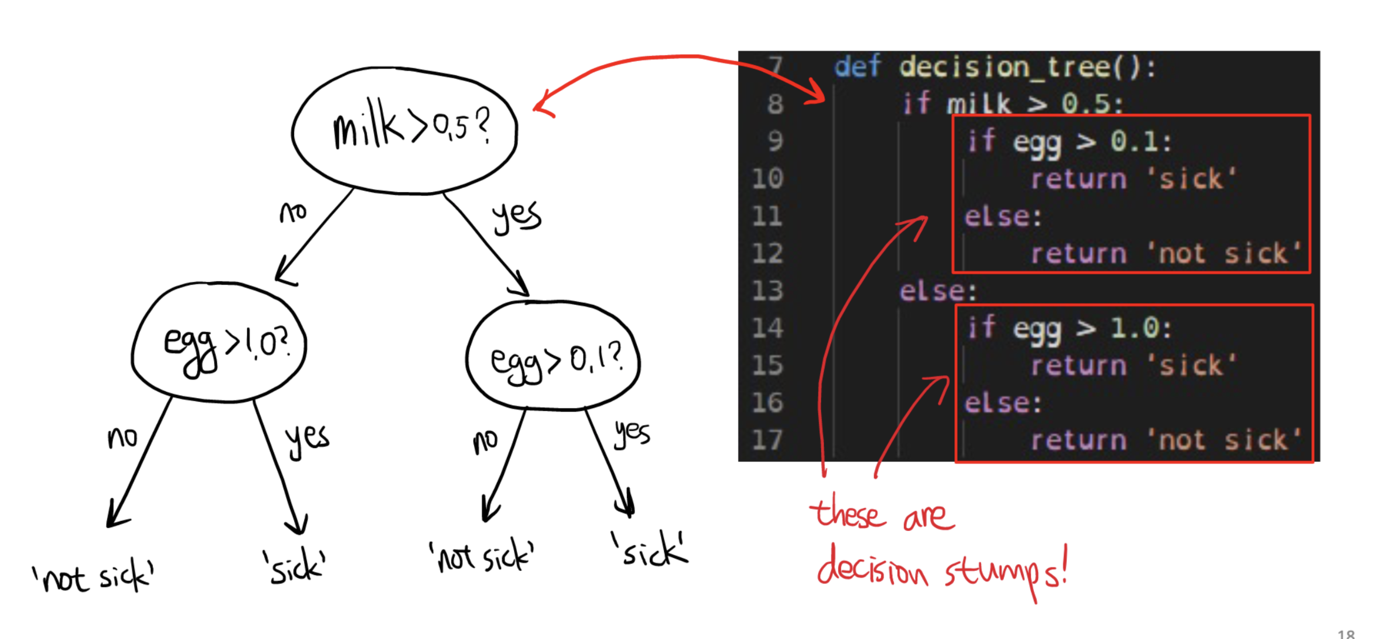
Decision Trees are simple proagrams consisting of:

A nested sequence of “if-else” decisions (splitting rules)
A class lable as return value

Example:

Decision Stump

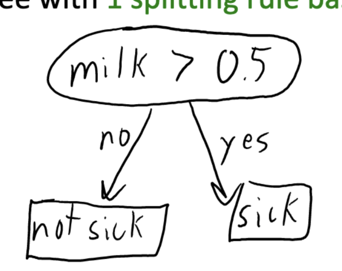
Decision Stump – A simple decision tree with 1 splitting rule based on 1 feature. Below is the sample of a decision stump:

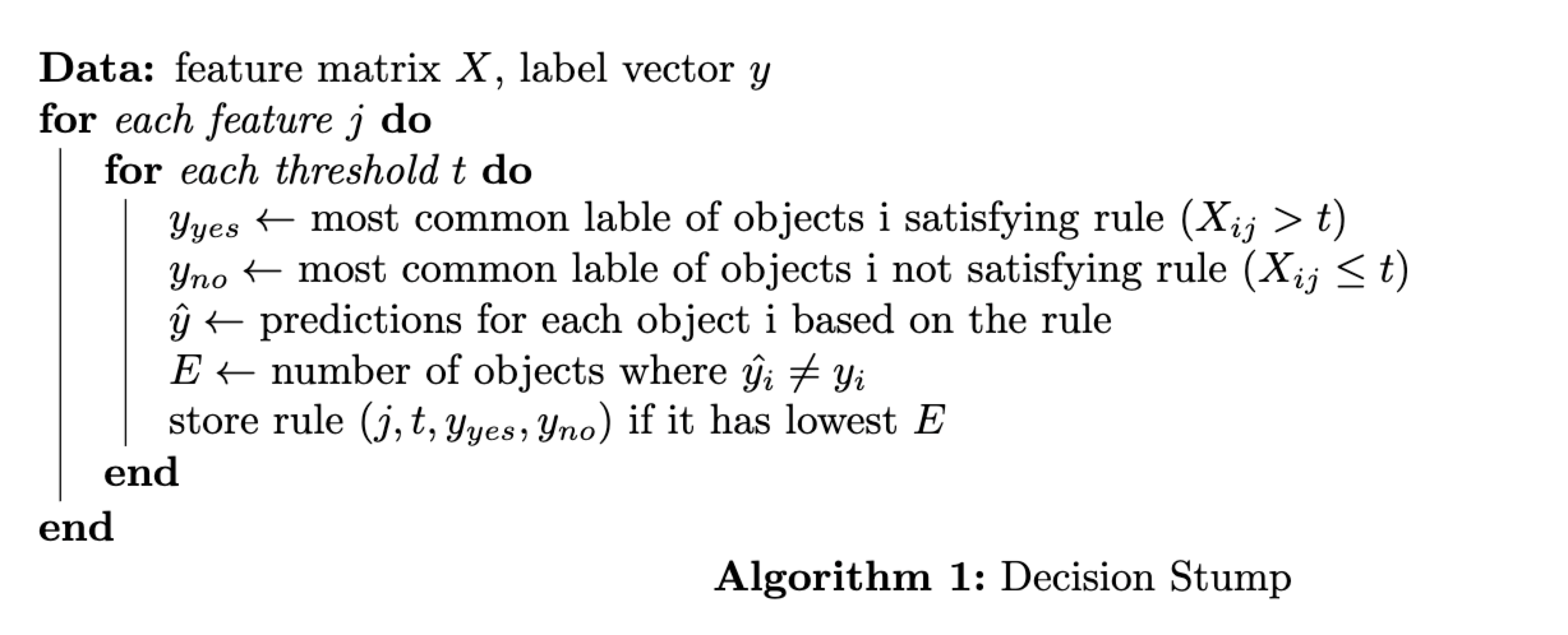
To learn a decision stump, we need to find 3 things:

which feature we should use to split data
what value should be used as threshold
what classes should we used for the leaves

Accuracy Score

To find out the best rule, we should define a score for each rule

The most intuitive score is classification accuray – if we use this rule, how many examples do we labe correctly?

Milk	Fish	Egg	Sick?
0.7	0	1	1
0.7	0	2	1
0	0	0	0
0.7	1.2	0	0
0	1.2	2	1
0	0	0	0

If we use below decision stump:

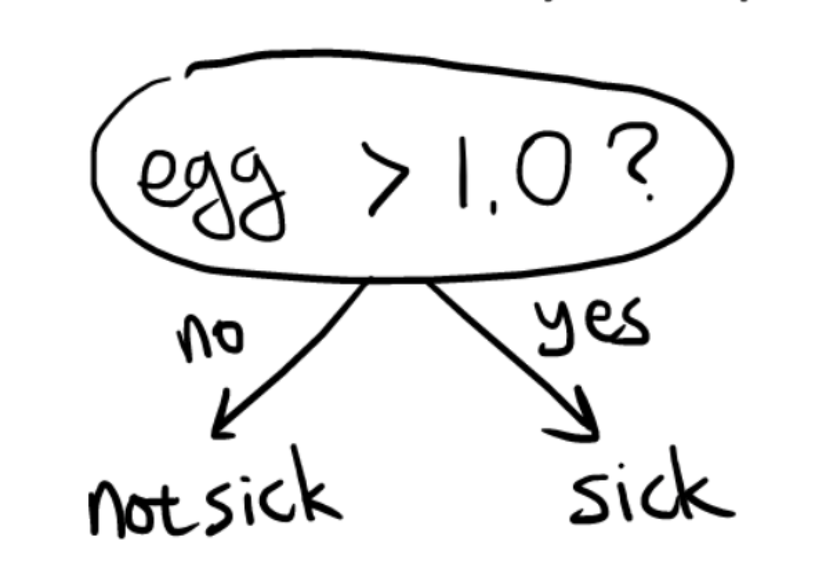
While egg > 1, sick: 2/2

egg <=1, not sick: 3/4

Accuracy: 5/6

We “learn” a decision stump by finding rule with the best score

Decision Stump Learning Pseudo-Code

Implementation

Github decision stump

Cost

n examples
d features
k threshholds (>0, >1, >2, …) for each feature

We have $O(dk)$ rules, and for each rule, we should go through n examples to find most common labels, then go through n examples again to compute the accuracy.
So the total cost is $O(ndk)$
If the features are binary, which means k =1, then the cost is $O(nd)$
However if features are numerical, then k = n, the cost is $O(n^2d)$

Decision Trees

Decision Stump VS Decison Trees

Decsion stumps have only one rule based on one feature, decision trees allow sequence of splits based on multiple features.

Decision Tree Learning - Greedy Recursive Splitting

Start with a full dataset, find the decision stump with the best score, split into 2 smaller datasets based on the stump.
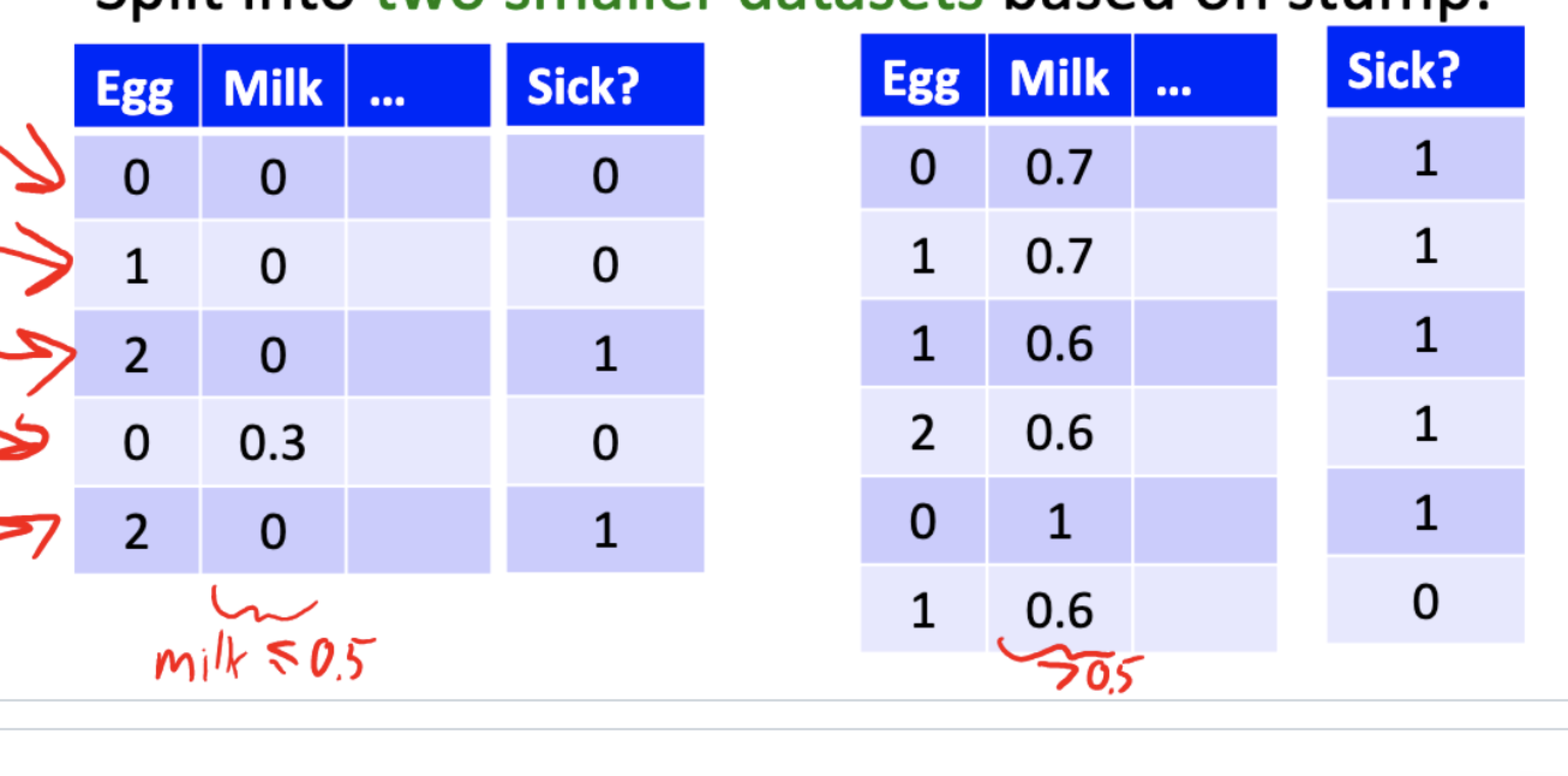
Now we have a decision stump and 2 sub-datasets. Fit a decision stump to each leaf’s data. And add these stumps to the tree

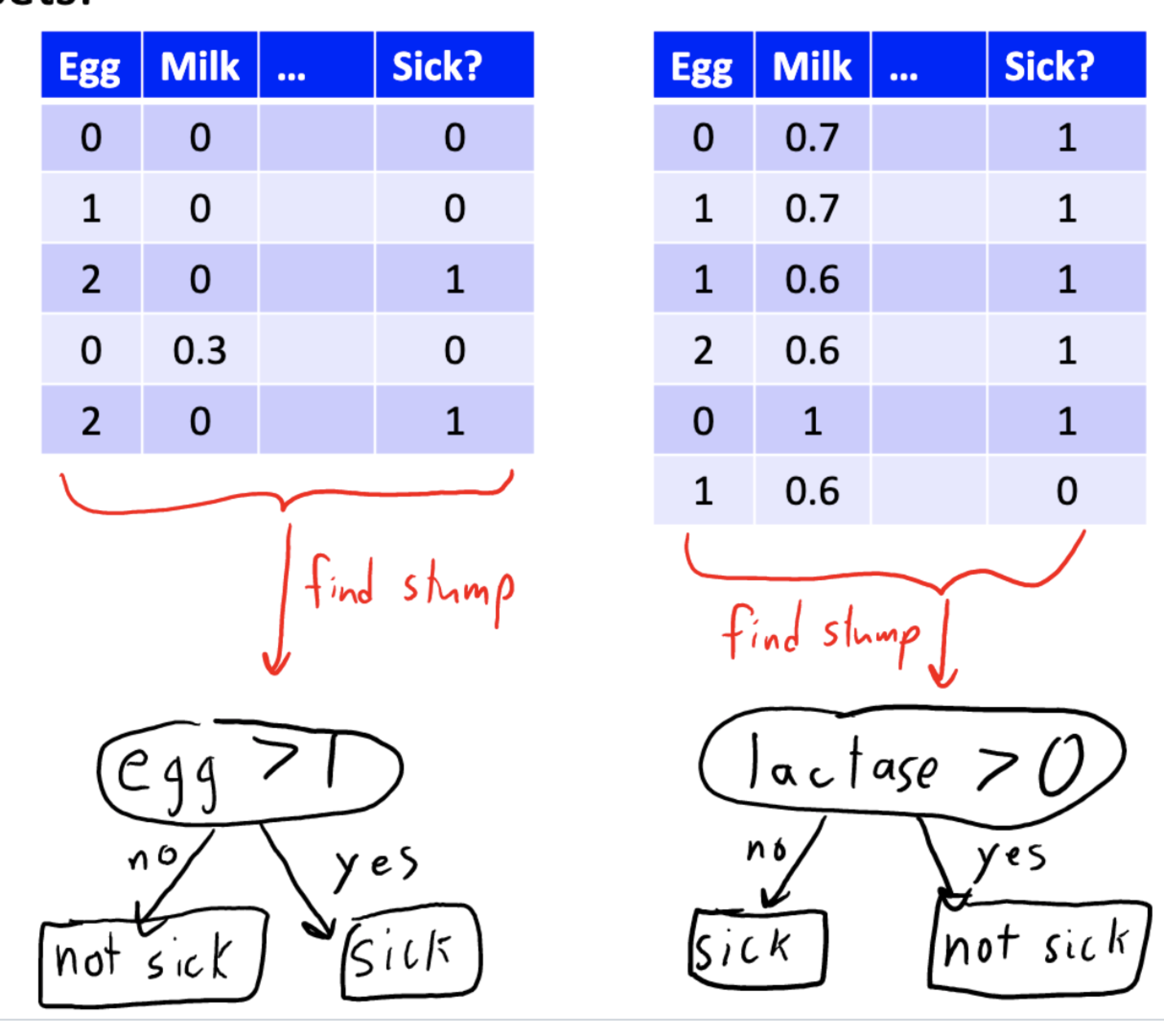
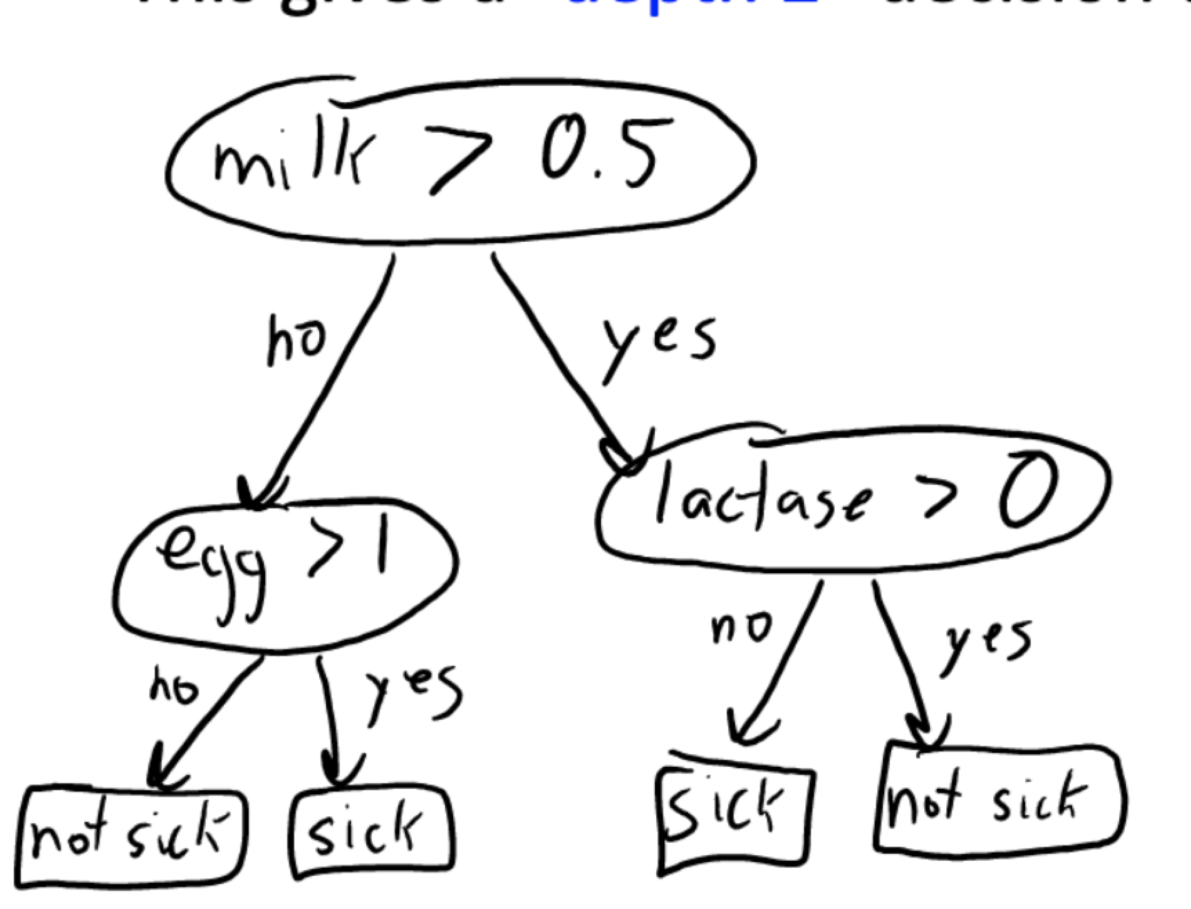
After adding stumps to the tree, we have a decision tree with depth 2:

It divide the original dataset as below subsets:

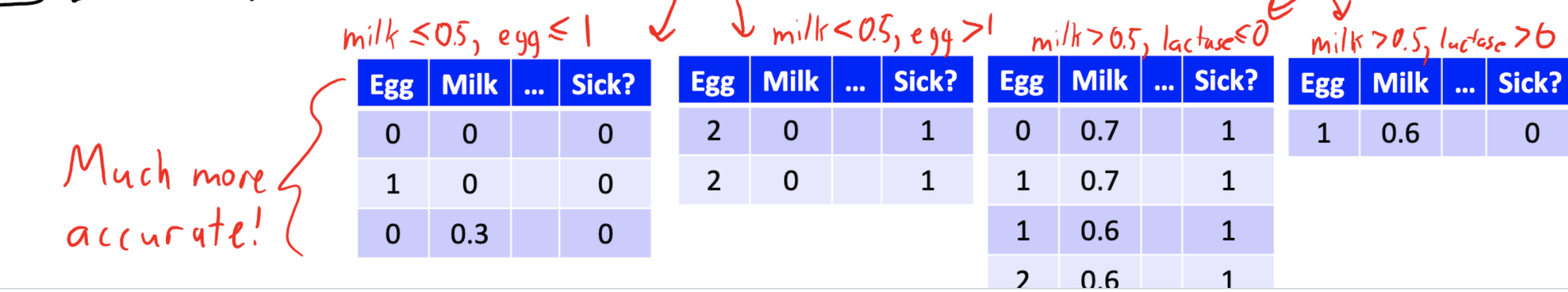
We might continue splitting until:

the leaves each has only one label.
we reach the defined maximum depth.

Score Function

We cannot use accuracy score:
for leafs: yes, just maximize accuracy
for internal nodes: not necessary
and maybe no simple rule like (egg >0.5) improves accuracy, but we should not stop.
(Example where accuracy fails can be found in the slides)

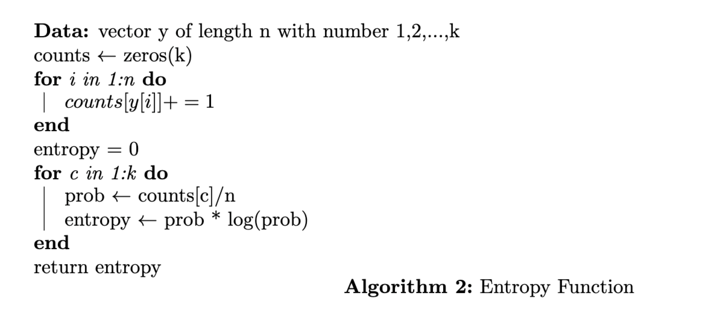
We can use the “information gain” as score function: choose split that decreases entropy of labels the most:

$information \space gain = entropy(y) - \frac{n_{yes}}{n}entropy(y_{yes}) - \frac{n_{no}}{n}entropy(y_{no})$

Infogain is large if labels are “more predictable” next layer.

Entropy Function

Code Implementation

We should use infogain as the score function.

class DecisionStumpInfoGain(DecisionStumpErrorRate):
    y_hat_yes = None
    y_hat_no = None
    j_best = None
    t_best = None

    def fit(self, X, y):
        n, d = X.shape
        class_count = np.unique(y).size
        self.y_hat_yes = utils.mode(y)
        
        # If all ys are the same
        if (class_count == 1):
            return
        p = np.bincount(y, minlength = class_count) / n
        prev_entropy = entropy(p)
        maxInfo = 0

        for j in range(d):
            thresholds = np.unique(X[:, j])
            for i in range(0, len(thresholds)):
                threshold = thresholds[i]

                y_yes = y[X[:, j] > threshold]
                p_yes = np.bincount(y_yes, minlength=class_count) / len(y_yes)
                y_yes_mode = utils.mode(y_yes)


                y_no = y[X[:, j] <= threshold]
                p_no = np.bincount(y_no, minlength=class_count) / len(y_no)
                y_no_mode = utils.mode(y_no)

                # Make prediction
                y_pred = y_yes_mode * np.ones(n)
                y_pred[X[:, j] <= threshold] = y_no_mode

                # score function
                new_entropy = len(y_yes) / n * entropy(p_yes) + len(y_no) / n * entropy(p_no)
                
                if prev_entropy - new_entropy > maxInfo:
                    maxInfo = prev_entropy - new_entropy
                    self.j_best = j
                    self.t_best = threshold
                    self.y_hat_yes = y_yes_mode
                    self.y_hat_no = y_no_mode

Then split recursively until the designed depth or it has already reached the best.

    def fit(self, X, y):
        # Fits a decision tree using greedy recursive splitting

        # Learn a decision stump
        stump_model = self.stump_class()
        stump_model.fit(X, y)

        if self.max_depth <= 1 or stump_model.j_best is None:
            # If we have reached the maximum depth or the decision stump does
            # nothing, use the decision stump

            self.stump_model = stump_model
            self.submodel_yes = None
            self.submodel_no = None
            return

        # Fit a decision tree to each split, decreasing maximum depth by 1
        j = stump_model.j_best
        value = stump_model.t_best

        # Find indices of examples in each split
        yes = X[:, j] > value
        no = X[:, j] <= value

        # Fit decision tree to each split
        self.stump_model = stump_model
        self.submodel_yes = DecisionTree(
            self.max_depth - 1, stump_class=self.stump_class
        )
        self.submodel_yes.fit(X[yes], y[yes])
        self.submodel_no = DecisionTree(
            self.max_depth - 1, stump_class=self.stump_class
        )
        self.submodel_no.fit(X[no], y[no])